Non-Intrusive Reduced-Order Modeling Using Uncertainty-Aware Deep Neural Networks and Proper Orthogonal Decomposition: Application to Flood Modeling

Authors

Pierre Jacquier, Azzedine Abdedou, Vincent Delmas, Azzeddine Soulaïmani

Abstract

Deep Learning research is advancing at a fantastic rate, and there is much to gain from transferring this knowledge to older fields like Computational Fluid Dynamics in practical engineering contexts. This work compares state-of-the-art methods that address uncertainty quantification in Deep Neural Networks, pushing forward the reduced-order modeling approach of Proper Orthogonal Decomposition-Neural Networks (POD-NN) with Deep Ensembles and Variational Inference-based Bayesian Neural Networks on two-dimensional problems in space. These are first tested on benchmark problems, and then applied to a real-life application: flooding predictions in the Mille Îles river in the Montreal, Quebec, Canada metropolitan area. Our setup involves a set of input parameters, with a potentially noisy distribution, and accumulates the simulation data resulting from these parameters. The goal is to build a non-intrusive surrogate model that is able to know when it doesn’t know, which is still an open research area in Neural Networks (and in AI in general). With the help of this model, probabilistic flooding maps are generated, aware of the model uncertainty. These insights on the unknown are also utilized for an uncertainty propagation task, allowing for flooded area predictions that are broader and safer than those made with a regular uncertainty-uninformed surrogate model. Our study of the time-dependent and highly nonlinear case of a dam break is also presented. Both the ensembles and the Bayesian approach lead to reliable results for multiple smooth physical solutions, providing the correct warning when going out-of-distribution. However, the former, referred to as POD-EnsNN, proved much easier to implement and showed greater flexibility than the latter in the case of discontinuities, where standard algorithms may oscillate or fail to converge.

Reduced Basis Generation with Proper Orthogonal Decomposition

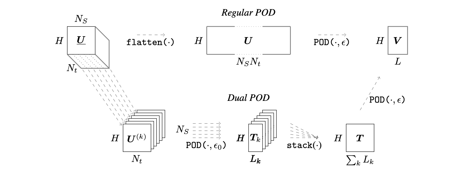
We start by defining $u$, our $\mathbb{R}^{D}$-valued function of interest. Computing this function is costly, so only a finite number $S$ of solutions called snapshots can be realized. In our applications, the spatial mesh of $N_D$ nodes is considered fixed in time, and since it is known and defined upfront, so we consider the number of outputs $H=N_D\times D$, the total number of degrees of freedom (DOFs) of the mesh. The simulation data, obtained from computing the function $u$ with $S$ parameter sets $\bm{s}^{(i)}$, is stored in a matrix of snapshots $\bm{U} = [u_D(\bm{s}^{(1)})|\ldots|u_D(\bm{s}^{(S)})] \in \mathbb{R}^{H \times S}$. Proper Orthogonal Decomposition (POD) is used to build a Reduced-Order Model (ROM) and produce a low-rank approximation, which will be much more efficient to compute and use when rapid multi-query simulations are required. With the snapshots method, a reduced POD basis can be efficiently extracted in a finite-dimension context. In our case, we begin with the $\bm{U}$ matrix, and use the Singular Value Decomposition algorithm, to extract $\bm{W} \in \mathbb{R}^{H \times H}$, $\bm{Z} \in \mathbb{R}^{S \times S}$ and the $r$ descending-ordered positive singular values matrix $\bm{D} = \text{diag}(\xi_1, \xi_2, \ldots, \xi_r)$ such that

\[ \begin{aligned} \bm{U} = \bm{W} \begin{bmatrix} \bm{D} & 0 \\ 0 & 0 \end{bmatrix} \bm{Z}^\intercal. \end{aligned} \]

For the finite truncation of the first $L$ modes, the following criterion on the singular values is imposed, with a hyperparameter $\epsilon$ given as

\[ \dfrac{\sum_{l=L+1}^{r} \xi_l^2}{\sum_{l=1}^{r} \xi_l^2} \leq \epsilon, \]

and then each mode vector $\bm{V}_j \in \mathbb{R}^{S}$ can be found from $\bm{U}$ and the $j$-th column of $\bm{Z}$, $\bm{Z}_j$, with

\[ \bm{V}_j = \dfrac{1}{\xi_j} \bm{U} \bm{Z}_j, \] so that we can finally construct our POD mode matrix

\[ \bm{V} = \left[\bm{V}_1 | \ldots | \bm{V}_j | \ldots | \bm{V}_L\right] \in \mathbb{R}^{H \times L}. \] To project to and from the low-rank approximation requires projection coefficients; those corresponding to the matrix of snapshots are obtained by the following

\[ \bm{v} = \bm{V}^\intercal \bm{U}, \] and then $\bm{U}_\textrm{POD}$, the approximation of $\bm{U}$, can be projected back to the expanded space:

\[ \bm{U}_\textrm{POD} = \bm{V}\bm{V}^\intercal\bm{U} = \bm{V} \bm{v}. \]

POD-EnsNN: Learning Expansion Coefficients Distributions using Deep Ensembles

Deep Neural Networks with built-in variance

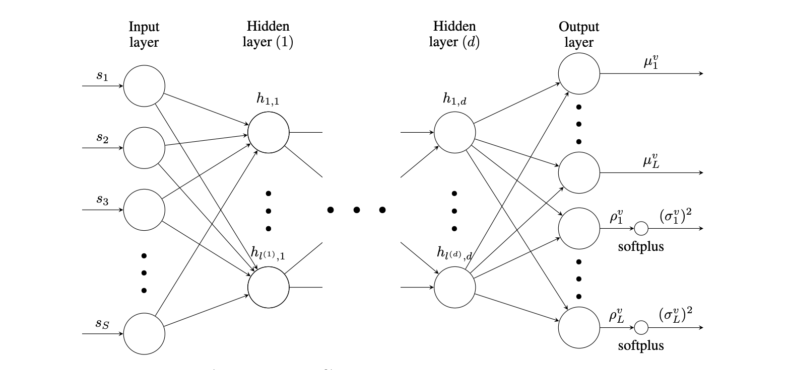
This statistical step is handled in the POD-NN framework by inferring the mapping with a Deep Neural Network, $\hat{u}_{DB}(\bm{s};\bm{w},\bm{b})$. The weights and biases of the network, $\bm{w}$ and $\bm{b}$, respectively, represent the model parameters and are learned during training (offline phase), to be later reused to make predictions (online phase). The network’s number of hidden layers is called the depth, $d$, which is chosen without accounting for the input and output layers. Each layer has a specific number of neurons that constitutes its width, $l^{(j)}$.

The main difference here with an ordinary DNN architecture for regression resides in the dual output, where the final layer size is twice the number of expansion coefficients to project, $l^{(d+1)}=2L$, since it outputs both a mean value $\bm{\mu}^v$ and a raw variance $\bm{\rho}^v$, which will then be constrained for positiveness through a softplus function, finally outputting ${\bm{\sigma^v}}^2$ as

\[ {\bm{\sigma}^v}^2 = \textrm{softplus}(\bm{\rho}^v) := \log(1 + \exp(\bm{\bm{\rho}^v})). \]

Since this predicted variance reports the spread, or noise, in data (the inputs’ data are drawn from a distribution), and so it would not be reduced even if we were to grow our dataset larger, it accounts for the aleatoric uncertainty, which is usually separated from epistemic uncertainty.

Ensemble training

Considering an $N$-sized training dataset $\mathcal{D}={\bm{X}_i, \bm{v}_i}$, with $\bm{X}_i$ denoting the normalized non-spatial parameters $\bm{s}$, and $\bm{v}_i$ the corresponding expansion coefficients from a training/validation-split of the matrix of snapshots $\bm{U}$, an optimizer performs several training epochs $N_e$ to minimize the following Negative Log-Likelihood loss function with respect to the network weights and biases parametrized by $\bm{\theta}=(\bm{w}, \bm{b})$

\[ \begin{aligned} \mathcal{L}_{\textrm{NLL}}(\mathcal{D},\bm{\theta}):=\dfrac{1}{N} \sum{i=1}^{N}\left[\dfrac{\log\ \bm{\sigma}{\bm{\theta}}^v(\bm{X}_i)^2}{2}+ \dfrac{(\bm{v}_i-\bm{\mu}^v{\bm{\theta}}(\bm{X}i))^2}{2 \bm{\sigma}{\bm{\theta}}^v(\bm{X}_i)^2}\right], \end{aligned} \]

with the normalized inputs $\bm{X}$, $\bm{\mu}^v_{\bm{\theta}}(\bm{X})$ and $\bm{\sigma}_{\bm{\theta}}^v(\bm{X})^2$ as the mean and variance, respectively, retrieved from the $\bm{\theta}$-parametrized network.

In practice, this loss gets an L2 regularization as an additional term, producing

\[ \begin{aligned} \mathcal{L}^\lambda_{\textrm{NLL}}(\mathcal{D}, \bm{\theta}):=\mathcal{L}_\textrm{NLL}(\mathcal{D}, \bm{\theta})+\lambda ||\bm{w}||^2.\end{aligned} \]

The idea behind Deep Ensembles is to randomly initialize $M$ sets of $\bm{\theta}_{m}=({\bm{w}},{\bm{b}})$, thereby creating $M$ independent neural networks (NNs). Each NN is then subsequently trained. Overall, the predictions moments in the reduced space $(\bm{\mu}^v_{\bm{\theta}_m},\bm{\sigma}^v_{\bm{\theta}_m})$ of each NN create a probability mixture, which, as suggested by the original authors, we can approximate in a single Gaussian distribution, leading to a mean expressed as

\[ \begin{aligned} \bm{\mu}^v_*(\bm{X}) = \dfrac{1}{M} \sum_{m=1}^{M}\bm{\mu}^v_{\bm{\theta}_m}(\bm{X}), \end{aligned} \] and a variance subsequently obtained as

\[ \bm{\sigma}^v_*(\bm{X})^2 = \dfrac{1}{M} \sum_{m=1}^{M} \left[\bm{\sigma}_{\bm{\theta}_m}^v(\bm{X})^2 + \bm{\mu}^v_{\bm{\theta}_m}(\bm{X})^2\right] - \bm{\mu}_*^v(\bm{X})^2. \]

The model is now accounting for the epistemic uncertainty through random initialization and variability in the training step. This uncertainty is directly linked to the model and could be reduced if we had more data. The uncertainty is directly related to the data-fitting capabilities of the model and thus will snowball in the absence of such data since there are no more constraints.

POD-BNN: Bayesian Neural Networks and Variational Inference as an Alternative

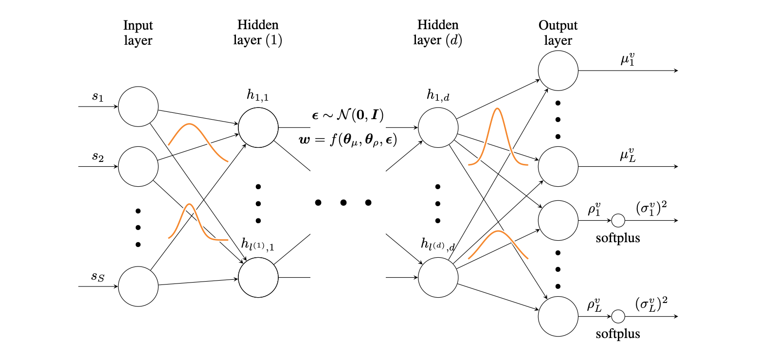For this model, the epistemic uncertainty treatment is very different. Earlier, even though the NNs were providing us with a mean and variance, they were still deterministic, and variability was obtained by assembling randomly initialized models. The Bayesian treatment instead aims to assign distributions according to the network’s weights, and so they therefore have a probabilistic output by design. Considering a dataset $\mathcal{D}={\bm{X}_i, \bm{v}_i}$, a likelihood function $p(\mathcal{D}|\bm{w})$ can be built, with $\bm{w}$ denoting both the weights $\bm{w}$ and the biases $\bm{b}$ for simplicity. The goal is then to construct a posterior distribution $p(\bm{w}|\mathcal{D})$ to achieve the following posterior predictive distribution on the target $\bm{v}$ for a new input $\bm{X}$

\[ p(\bm{v}|\bm{X},\mathcal{D})=\int p(\bm{v}|\bm{X},\bm{w})p(\bm{w}|\mathcal{D})\,d\bm{w}, \]

which cannot be achieved directly in a NN context, due to the infinite possibilities for the weights $\bm{w}$, leaving the posterior $p(\bm{w}|\mathcal{D})$ intractable.

Variational inference aims at construction an approximate posterior distribution $q(\bm{w}|\bm{\theta})$, by minimizing the KL divergence with the real posterior. In our case, it writes as $\textrm{KL}(q(\bm{w}|\bm{\theta}),||p(\bm{w}|\mathcal{D}))$ with respect to the new parameters $\bm{\theta}$ called latent variables, such as

\[ \begin{aligned} \textrm{KL}(q(\bm{w} | \bm{\theta}) || p(\bm{w} | \mathcal{D})) &= \int q(\bm{w} | \bm{\theta}) \log \dfrac{q(\bm{w} | \bm{\theta})}{p(\bm{w}|\mathcal{D})}\, d\bm{w}=\mathbb{E}_{q(\bm{w} | \bm{\theta})}\log \dfrac{q(\bm{w} | \bm{\theta})}{p(\bm{w}|\mathcal{D})},\end{aligned} \] which can be show to written as

\[ \begin{aligned} \textrm{KL}(q(\bm{w} | \bm{\theta}) || p(\bm{w} | \mathcal{D})) &=\textrm{KL}(q(\bm{w}|\bm{\theta})||p(\bm{w})) - \mathbb{E}_{q(\bm{w} | \bm{\theta})} \log p(\mathcal{D}|\bm{w}) + \log p(\mathcal{D})\\ &=:\mathcal{F}(\mathcal{D},\bm{\theta}) + \log p(\mathcal{D}) \end{aligned} \]

The term $\mathcal{F}(\mathcal{D}, \bm{\theta})$ is commonly known as the variational free energy, and minimizing it with respect to the weights does not involve the last term $\log p(\mathcal{D})$, and so it is equivalent to the goal of minimizing $\textrm{KL}(q(\bm{w}|\bm{\theta}),||p(\bm{w}|\mathcal{D}))$. If an appropriate choice of $q$ is made, the predictive posterior can become computationally tractable.

By drawing $N_\textrm{mc}$ samples $\bm{w}^{(i)}$ from the distribution $q(\bm{w}|\bm{\theta})$ at the layer level, it is possible to construct a tractable Monte-Carlo approximation of the variational free energy, such as

\[ \mathcal{F}(\mathcal{D},\bm{\theta}) \approx \sum_{i=1}^{N_\textrm{mc}} \left[ \log q(\bm{w}^{(i)} | \bm{\theta}) - \log p(\bm{w}^{(i)})\right] - \sum_{m=1}^{N} \log p(\mathcal{D} | \bm{w}_m), \] with $p(\bm{w}^{(i)})$ denoting the prior on the drawn weight $\bm{w}^{(i)}$, which is chosen by the user. The last term shows to be approximated by summing on the $N$ samples at the output level (for each training input).

A Few Results

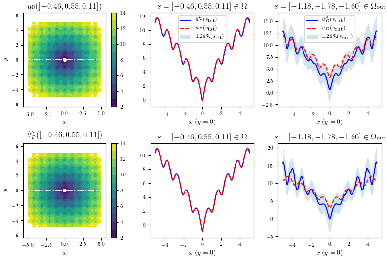
Benchmark: 2D Ackley Function

To test the methods, one of the chosen benchmark was a stochastic version of Ackley Function. The following result show the predictions in the second and third column, respectively, in and out of the training scope. We see the uncertainties correctly snowballing in the latter.

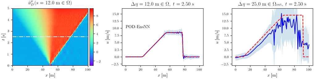
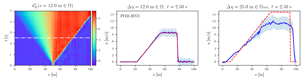
POD-EnsNN 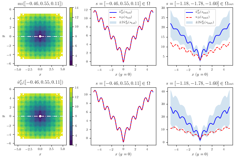POD-BNN

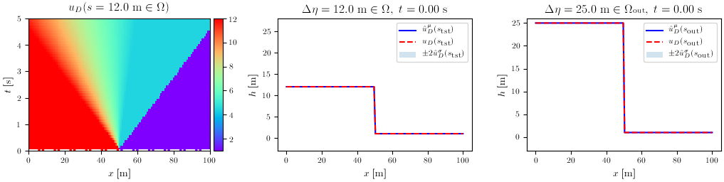
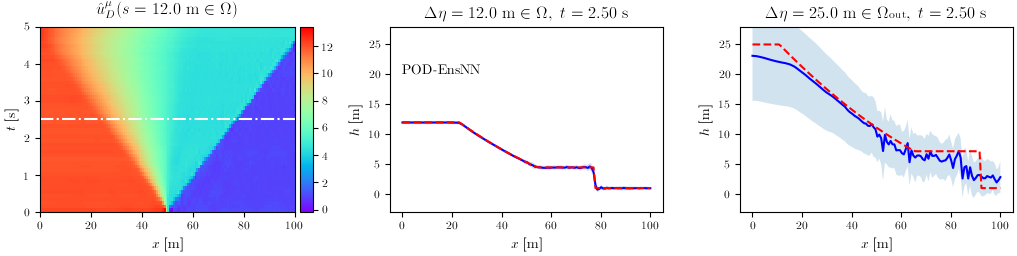
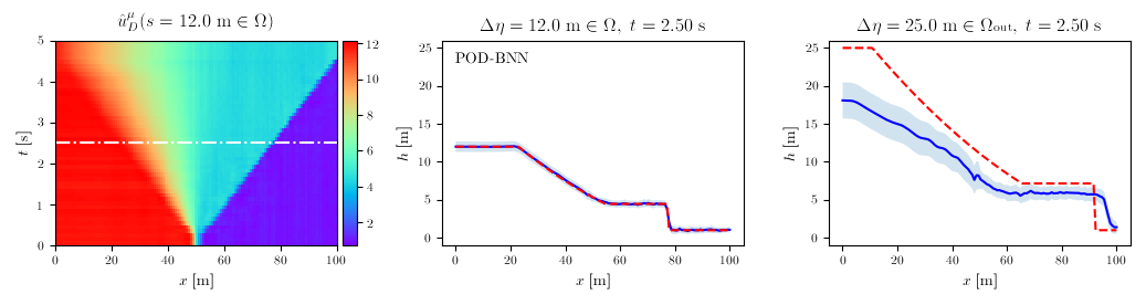
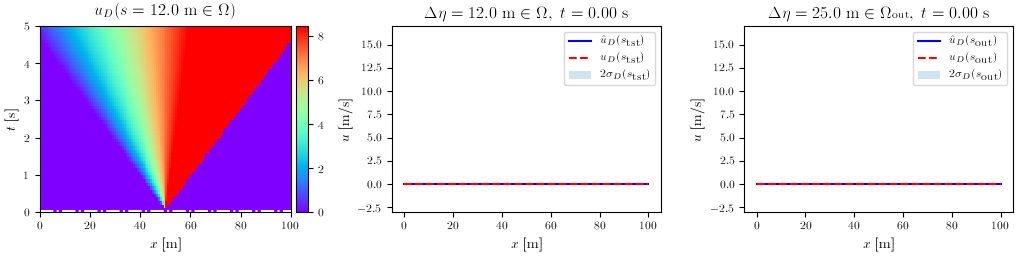
Shallow Water equations validation: 1D dam break

The final validation case was a 1D, time-unsteady problem involving the equations of interest in flood modeling: the Shallow Water Equations. In this case, the POD handles 2 DOFs per node, the water depth $h$ and the velocity $u$. For both, the results are displayed for the two methods, with the second and third column denoting again in- and out-of-distribution input parameters.

Water depth $h$ Velocity $u$

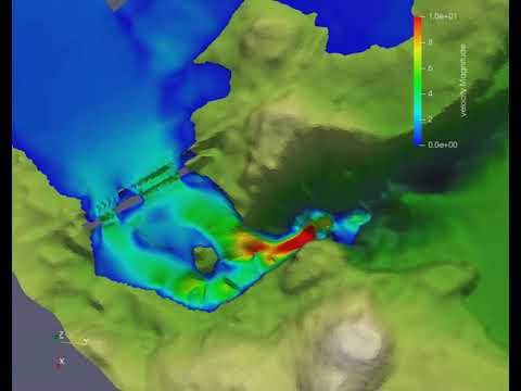
Rendering training data from CuteFlow, our numerical solver

In the following video, we render using the visualization software ParaView one of the snapshot, representing the training data in the case of a dam break, here on dry soil.

For more details and results, please check out the full paper.

Acknowledgements

This research was enabled in part by funding from the National Sciences and Engineering Research Council of Canada and Hydro-Québec; by bathymetry data from the Communauté métropolitaine de Montréal; and by computational support from Calcul Québec and Compute Canada.

Citation

@misc{jacquier2020nonintrusive,
    title={Non-Intrusive Reduced-Order Modeling Using Uncertainty-Aware Deep Neural Networks and Proper Orthogonal Decomposition: Application to Flood Modeling},
    author={Pierre Jacquier and Azzedine Abdedou and Vincent Delmas and Azzeddine Soulaimani},
    year={2020},
    eprint={2005.13506},
    archivePrefix={arXiv},
    primaryClass={physics.comp-ph}
}